LinuxCNC S-Curve Accelerations

arvidb
Offline
Platinum Member

14 Jun 2021 12:16 #212023 by arvidb

Replied by arvidb on topic LinuxCNC S-Curve Accelerations

Hehe, maybe I'm a bit of a perfectionist?

(Yes I am...)

But even if you did modify only the acc-cmd, how would you use it to control your machine? If I'm not mistaken, pretty much all configs use the motor-pos-cmd as the setpoint for the PID controller (that then outputs a velocity command to +/-10 V outputs, or to stepgens). So you really do need to have the pos-cmd itself change in a way that doesn't lead to infinite jerk.

Please Log in or Create an account to join the conversation.

Grotius
Offline
Platinum Member

14 Jun 2021 12:42 - 14 Jun 2021 12:54 #212025 by Grotius

Replied by Grotius on topic LinuxCNC S-Curve Accelerations

Hi,

The problem of c coding or mathematical knowledge is solved.
Attached a component that uses a scurve header only library.
#include "scurve.h" to your component or c code or c++ code.

I think with this example users can retrieve all the info related to the scurve's acc, dcc, timestamp points, etc.
For interpolating on arc's just give the arclenght to the function. And then interpolate the result to the arc bow.
This can be done by % pathlenght interpolation.

The output is printed with rtapi into the terminal. This is done by setting the debug to 1.

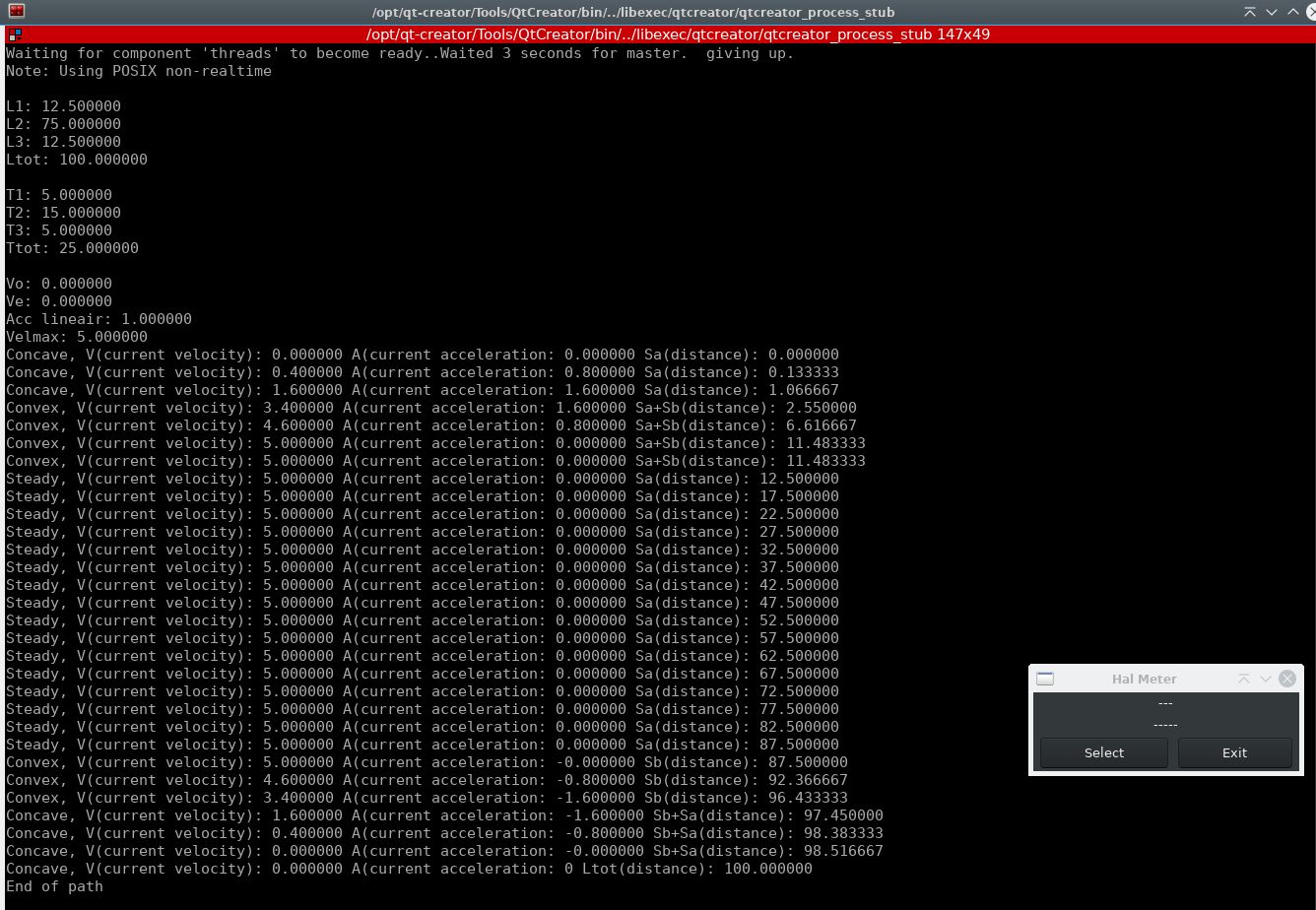
The function call from the component, wich is a line (path) of 100mm :

scurve(5,  // velmax
               1,   // accmax
               0,   // vo
               0,   // ve
               0,   // xs 
               0,   // ys
               0,   // zs
               100, // xe
               0,   // ye
               0,   // ze
               1, // time output resolution in sec, for example 0.001 is a point every ms
               1);  // debug 0 or 1

Rtapi result :

Now you can imagine what to do. Just play around with the code.
It has jerk, initial velocity and end velocity implemented. It has also a sampler if max velocity can not be reached.

Attached code is a "c kernel style" derivate from my original work at : github.com/grotius-cnc/S-curve-motion-pl...g/releases/tag/1.0.1

test.c

Warning: Spoiler!

/* Autogenerated by /opt/linuxcnc/bin/halcompile on Sun Jun 13 16:30:04 2021 -- do not edit */
#include "rtapi.h"
#ifdef RTAPI
#include "rtapi_app.h"
#endif
#include "rtapi_string.h"
#include "rtapi_errno.h"
#include "hal.h"
#include "rtapi_math64.h"
#include "scurve.h"

static int comp_id;

#ifdef MODULE_INFO
MODULE_INFO(linuxcnc, "component:test:test component");
MODULE_INFO(linuxcnc, "descr:\nTest Component\n\nCompile slogan :\n/opt/linuxcnc/bin/halcompile --compile /opt/linuxcnc/src/hal/components/test.comp\n\nPreprocess slogan :\n/opt/linuxcnc/bin/halcompile --preprocess /opt/linuxcnc/src/hal/components/test.comp\n\nThen copy it to the rtlib.\n\nThen in halview : loadrt test\n\n");
MODULE_INFO(linuxcnc, "author:Skynet");
MODULE_INFO(linuxcnc, "license:GPLv2 or greater");
MODULE_INFO(linuxcnc, "pin:enable:bit:0:in::None:None");
MODULE_INFO(linuxcnc, "pin:value:float:0:out::None:None");
MODULE_INFO(linuxcnc, "funct:_:1:");
MODULE_LICENSE("GPLv2 or greater");
#endif // MODULE_INFO

struct __comp_state {
    struct __comp_state *_next;
    hal_bit_t *enable;
    hal_float_t *value;
};
struct __comp_state *__comp_first_inst=0, *__comp_last_inst=0;

static void _(struct __comp_state *__comp_inst, long period);
static int __comp_get_data_size(void);
#undef TRUE
#define TRUE (1)
#undef FALSE
#define FALSE (0)
#undef true
#define true (1)
#undef false
#define false (0)

static int export(char *prefix, long extra_arg) {
    char buf[HAL_NAME_LEN + 1];
    int r = 0;
    int sz = sizeof(struct __comp_state) + __comp_get_data_size();
    struct __comp_state *inst = hal_malloc(sz);
    memset(inst, 0, sz);
    r = hal_pin_bit_newf(HAL_IN, &(inst->enable), comp_id,
        "%s.enable", prefix);
    if(r != 0) return r;
    r = hal_pin_float_newf(HAL_OUT, &(inst->value), comp_id,
        "%s.value", prefix);
    if(r != 0) return r;
    rtapi_snprintf(buf, sizeof(buf), "%s", prefix);
    r = hal_export_funct(buf, (void(*)(void *inst, long))_, inst, 1, 0, comp_id);
    if(r != 0) return r;
    if(__comp_last_inst) __comp_last_inst->_next = inst;
    __comp_last_inst = inst;
    if(!__comp_first_inst) __comp_first_inst = inst;
    return 0;
}
int rtapi_app_main(void) {
    int r = 0;
    comp_id = hal_init("test");
    if(comp_id < 0) return comp_id;
    r = export("test", 0);
    if(r) {
        hal_exit(comp_id);
    } else {
        hal_ready(comp_id);
    }
    return r;
}

void rtapi_app_exit(void) {

    hal_exit(comp_id);
}

#undef FUNCTION
#define FUNCTION(name) static void name(struct __comp_state *__comp_inst, long period)
#undef EXTRA_SETUP
#define EXTRA_SETUP() static int extra_setup(struct __comp_state *__comp_inst, char *prefix, long extra_arg)
#undef EXTRA_CLEANUP
#define EXTRA_CLEANUP() static void extra_cleanup(void)
#undef fperiod
#define fperiod (period * 1e-9)
#undef enable
#define enable (0+*__comp_inst->enable)
#undef value
#define value (*__comp_inst->value)


#line 33 "/opt/linuxcnc/src/hal/components/test.comp"

#include "rtapi_math.h"

FUNCTION(_) {
    if(enable){
    }

    if(value==0){
        scurve(5,  // velmax
               1,   // accmax
               0,   // vo
               0,   // ve
               0,   // xs
               0,   // ys
               0,   // zs
               100, // xe
               0,   // ye
               0,   // ze
               1, // time output resolution in sec, for example 0.001 is a point every ms
               1);  // debug 0 or 1
    }
    value=1;

}

static int __comp_get_data_size(void) { return 0; }

scurve.h

Warning: Spoiler!

#ifndef SCURVE_H
#define SCURVE_H

#include "rtapi.h"          /* RTAPI realtime OS API */
#include "rtapi_app.h"		/* RTAPI realtime module decls */
#include "math.h"           /* Used for pow and sqrt */

// With qt always do a make clean before a compile.

// Example function:
void myfirstvoid(float a, float b, float *result);

void myfirstvoid(float a, float b, float *result){
    *result=a+b;
}

// Data structures:

struct point {
    double x,y,z;
};

struct line {
    double xs,ys,zs;  //startpos
    double xe,ye,ze;  //endpos
    double lenght;    //lenght of primitive.
};

struct traject {

    double Vo;            //start velocity
    double Ve;            //end velocity
    double Vm;            //max velocity if atspeed can not be reached
    double Vel;           //feedrate - velocity
    double Acc_lineair;   //lineair acceleration, mm/sec^2
    double Acc_inflation; //max acceleration at inflection point, acc_lin*2, mm/sec^2

    double T1;            //total Acc time.
    double T2;            //total atspeed time.
    double T3;            //total Dcc time.
    double Ttot;          //total traject time, T1+T2+T3
    double T1h;           //total half Acc time, time to inflection point.
    double T3h;           //total half Dcc time, time to inflection point.

    double L1;            //acceleration lenght
    double L2;            //atspeed lenght.
    double L3;            //deacceleration lenght
    double Ltot;          //total traject lenght, L1+L2+L3
    double Li;            //line-line intersection x-value

    double Jm;            //max jerk for profile, x*acc_infl/T1 or T3

    struct line line;
};

// Declarations:

// Driver:
void scurve(double velmax,
            double accmax,
            double vo,
            double ve,
            double xs, double ys, double zs,    // Line startpoint
            double xe, double ye, double ze,    // Line endpoint
            double timeresolution,              // 0.001 for ms.
            int debug );                        // 0 or 1

struct traject TrajectCalculator(double Vel, double Acc, double Vo, double Ve, struct line line, int debug);   // First calculate classical lineair way
struct traject ScurveUp(struct traject tr, double timeresolution, int debug);
struct traject ScurveSteady(struct traject tr, double timeresolution, int debug);
struct traject ScurveDown(struct traject tr, double timeresolution, int debug);

// Functions:

void scurve(double velmax, double accmax, double vo, double ve, double xs, double ys, double zs, double xe, double ye, double ze, double timeresolution, int debug){

    struct line line;
    line.xs=xs; line.ys=ys; line.zs=zs;
    line.xe=xe; line.ye=ye; line.ze=ze;

    struct traject traject;

    // Add traject properties and calculate traject interval
    traject = TrajectCalculator(velmax,
                                accmax,
                                vo,
                                ve,
                                line,
                                debug);     // debug 0 or 1

    // Calculate Scurve
    ScurveUp(traject, timeresolution, debug);
    ScurveSteady(traject, timeresolution, debug);
    ScurveDown(traject, timeresolution, debug);
}

struct traject TrajectCalculator(double Vel, double Acc, double Vo, double Ve, struct line line, int debug){

    struct traject tr;
    // Data.
    tr.Vel=Vel;
    tr.Vo=Vo;
    tr.Ve=Ve;
    tr.Acc_lineair=Acc;

    // Formula.
    tr.Acc_inflation=tr.Acc_lineair*2;                      // Acceleration at s-curve inflation point = normal acceleration*2.
    tr.Ltot=sqrt(pow(line.xe-line.xs,2)+pow(line.ye-line.ys,2)+pow(line.ze-line.zs,2));
    tr.line.lenght=tr.Ltot; // Copy above lenght value.

    // Acc path.
    tr.T1=(tr.Vel-tr.Vo)/tr.Acc_lineair;
    tr.L1=0.5*tr.Acc_lineair*pow(tr.T1,2);

    // Dcc path.
    tr.T3=(tr.Vel-tr.Ve)/tr.Acc_lineair;                    // We could use a seperate dcc value.
    tr.L3=0.5*tr.Acc_lineair*pow(tr.T3,2);

    // At speed path.
    tr.L2=tr.Ltot-tr.L1-tr.L3;
    tr.T2=tr.L2/tr.Vel;


    // Motion can not reach full speed, find acc dcc intersection.
    if(tr.L2<0){
        // Decrease Velocity until L2 is positive, if Acceleration stays the same value.
        double TempVel=tr.Vel;
        for(double i=TempVel; i>0; i-=0.1){

            tr.Vel=i;
            //std::cout<<"Vel:"<<tr.Vel<<std::endl;

            // Acc path.
            tr.T1=(tr.Vel-tr.Vo)/tr.Acc_lineair;
            tr.L1=0.5*tr.Acc_lineair*pow(tr.T1,2);

            // Dcc path.
            tr.T3=(tr.Vel-tr.Ve)/tr.Acc_lineair;            // We could use a seperate dcc value.
            tr.L3=0.5*tr.Acc_lineair*pow(tr.T3,2);

            // At speed path.
            tr.L2=tr.Ltot-tr.L1-tr.L3;
            tr.T2=tr.L2/tr.Vel;

            if(tr.L2>=0){

                //ui->doubleSpinBox_velocity_max->setValue(i);
                break;
            }
        }
    }

    tr.Ttot=tr.T1+tr.T2+tr.T3;
    tr.T1h=tr.T1/2;
    tr.T3h=tr.T3/2;

    if(debug){
        rtapi_print_msg(RTAPI_MSG_INFO,"TRAJECT CALCULATOR \n");
        rtapi_print_msg(RTAPI_MSG_ERR,"L1: %f \n", tr.L1);
        rtapi_print_msg(RTAPI_MSG_ERR,"L2: %f \n", tr.L2);
        rtapi_print_msg(RTAPI_MSG_ERR,"L3: %f \n", tr.L3);
        rtapi_print_msg(RTAPI_MSG_ERR,"Ltot: %f \n", tr.Ltot);
        rtapi_print_msg(RTAPI_MSG_ERR,"\n");
        rtapi_print_msg(RTAPI_MSG_ERR,"T1: %f \n", tr.T1);
        rtapi_print_msg(RTAPI_MSG_ERR,"T2: %f \n", tr.T2);
        rtapi_print_msg(RTAPI_MSG_ERR,"T3: %f \n", tr.T3);
        rtapi_print_msg(RTAPI_MSG_ERR,"Ttot: %f \n", tr.Ttot);
        rtapi_print_msg(RTAPI_MSG_ERR,"\n");
        rtapi_print_msg(RTAPI_MSG_ERR,"Vo: %f \n", tr.Vo);
        rtapi_print_msg(RTAPI_MSG_ERR,"Ve: %f \n", tr.Ve);
        rtapi_print_msg(RTAPI_MSG_ERR,"Acc lineair: %f \n", tr.Acc_lineair);
        rtapi_print_msg(RTAPI_MSG_ERR,"Velmax: %f \n", tr.Vel);
    }

    return tr;
}

struct traject ScurveUp(struct traject tr, double timeresolution, int debug){

    double A=0;                                     // Current acceleration.
    double V=0;                                     // Current velocity.
    double t=0;                                     // Time.
    double Jm=0;                                    // Max Jerk for profile, 2*Ainfl/T <= Jm.
    double Sa=0;                                    // Concave distance.
    double Sb=0;                                    // Convex distance.

    for(double T=0; T<=tr.T1; T+=timeresolution){

        Jm = 2*tr.Acc_inflation/tr.T1;

        if(T<(tr.T1/2)){

            t=T;

            V = Jm*(t*t)/2;
            V+=tr.Vo;                               // Add initial velocity.
            A = Jm*t;
            Sa = 0*t + Jm*(t*t*t)/6;

            struct point p;
            p.x=tr.line.xs+((tr.line.xe-tr.line.xs)*(Sa/tr.line.lenght));
            p.y=tr.line.ys+((tr.line.ye-tr.line.ys)*(Sa/tr.line.lenght));
            p.z=tr.line.zs+((tr.line.ze-tr.line.zs)*(Sa/tr.line.lenght));
            //pointvec.push_back(p);         // Store the path point every 1ms, t=0.001

            if(debug){
                rtapi_print_msg(RTAPI_MSG_ERR,"Concave, V(current velocity): %f A(current acceleration: %f Sa(distance): %f \n", V, A, Sa);
            }
        }

        if(T>(tr.T1/2) && T<=(tr.T1)){

            t=tr.T1h-(T-(0.5*tr.T1));               // T inverted

            V = Jm*(t*t)/2;
            V = tr.Vel-V;                           // Mirror
            A = Jm*t;

            t=T-(0.5*tr.T1);                        // T non inverted
            Sb = Jm*(tr.T1h*tr.T1h)/2*t + tr.Acc_inflation*(t*t)/2 -Jm*(t*t*t)/6;

            struct point p;
            p.x=tr.line.xs+((tr.line.xe-tr.line.xs)*((Sa+Sb)/tr.line.lenght));
            p.y=tr.line.ys+((tr.line.ye-tr.line.ys)*((Sa+Sb)/tr.line.lenght));
            p.z=tr.line.zs+((tr.line.ze-tr.line.zs)*((Sa+Sb)/tr.line.lenght));
            //pointvec.push_back(p);         // Store the path point every 1ms, t=0.001

            if(debug){
                rtapi_print_msg(RTAPI_MSG_ERR,"Convex, V(current velocity): %f A(current acceleration: %f Sa+Sb(distance): %f \n", V, A, Sa+Sb);
            }
        }
    }

    struct point p;
    p.x=tr.line.xs+((tr.line.xe-tr.line.xs)*((Sa+Sb)/tr.line.lenght));
    p.y=0;
    p.z=0;
    //pointvec.push_back(p);         // Store the path point every 1ms, t=0.001

    if(debug){
        rtapi_print_msg(RTAPI_MSG_ERR,"Convex, V(current velocity): %f A(current acceleration: %f Sa+Sb(distance): %f \n", V, A, Sa+Sb);
    }

    return tr;
}

struct traject ScurveSteady(struct traject tr, double timeresolution, int debug){

    double A=0;                                     // Current acceleration.
    double V=0;                                     // Current velocity.
    double S=0;                                     // S(t) distance.

    for(double T=tr.T1; T<=tr.T1+tr.T2; T+=timeresolution){

        V=tr.Vel;
        A=0;
        //S=(tr.Vel*T)-tr.L1;

        S=tr.L1+((T-tr.T1)*tr.Vel);
        // Todo=Sa/tr.Ltot;                     // Point on path ratio.

        struct point p;
        p.x=tr.line.xs+((tr.line.xe-tr.line.xs)*(S/tr.line.lenght));
        p.y=tr.line.ys+((tr.line.ye-tr.line.ys)*(S/tr.line.lenght));
        p.z=tr.line.zs+((tr.line.ze-tr.line.zs)*(S/tr.line.lenght));
        //pointvec.push_back(p);         // Store the path point every 1ms, t=0.001

        if(debug){
            rtapi_print_msg(RTAPI_MSG_ERR,"Steady, V(current velocity): %f A(current acceleration: %f Sa(distance): %f \n", V, A, S);
        }
    }
    return tr;
}

struct traject ScurveDown(struct traject tr, double timeresolution, int debug){

    double A=0;                                     // Current acceleration.
    double V=0;                                     // Current velocity.
    double t=0;                                     // Time.
    double Jm=0;                                    // Max Jerk for profile, 2*Ainfl/T <= Jm.
    double Sa=0;                                    // Concave distance.
    double Sb=0;                                    // Convex distance.

    for(double T=tr.T1+tr.T2; T<=tr.Ttot; T+=timeresolution){

        Jm = 2*tr.Acc_inflation/tr.T3;

        if(T<(tr.T1+tr.T2+tr.T3h)){

            t=T-tr.T1-tr.T2;

            V = Jm*(t*t)/2;
            V = tr.Vel-V;                           // Mirror
            A = -fabs(Jm*t);

            t=tr.T3h;
            double Sbmax=Jm*(tr.T3h*tr.T3h)/2*t + tr.Acc_inflation*(t*t)/2 -Jm*(t*t*t)/6;

            t=T-tr.T1-tr.T2;
            t=tr.T3h-t;

            Sb = Sbmax-( Jm*(tr.T3h*tr.T3h)/2*t + tr.Acc_inflation*(t*t)/2 -Jm*(t*t*t)/6 );
            Sb+= tr.L1+tr.L2;

            struct point p;
            p.x=tr.line.xs+((tr.line.xe-tr.line.xs)*(Sb/tr.line.lenght));
            p.y=tr.line.ys+((tr.line.ye-tr.line.ys)*(Sb/tr.line.lenght));
            p.z=tr.line.zs+((tr.line.ze-tr.line.zs)*(Sb/tr.line.lenght));
            //pointvec.push_back(p);         // Store the path point every 1ms, t=0.001

            if(debug){
                rtapi_print_msg(RTAPI_MSG_ERR,"Convex, V(current velocity): %f A(current acceleration: %f Sb(distance): %f \n", V, A, Sb);
            }
        }

        if(T>tr.T1+tr.T2+tr.T3h){

            t=T-tr.T1-tr.T2-tr.T3h;
            t=tr.T3h-t;

            V = Jm*(t*t)/2;
            V+=tr.Ve;
            A = -fabs(Jm*t);

            t=tr.T3h;
            double SaMax =  0*t + Jm*(t*t*t)/6;

            t=T-tr.T1-tr.T2-tr.T3h;
            t=tr.T3h-t; // Mirror
            Sa = SaMax-( 0*t + Jm*(t*t*t)/6);

            struct point p;
            p.x=tr.line.xs+((tr.line.xe-tr.line.xs)*((Sb+Sa)/tr.line.lenght));
            p.y=tr.line.ys+((tr.line.ye-tr.line.ys)*((Sb+Sa)/tr.line.lenght));
            p.z=tr.line.zs+((tr.line.ze-tr.line.zs)*((Sb+Sa)/tr.line.lenght));
            //pointvec.push_back(p);         // Store the path point every 1ms, t=0.001

            if(debug){
                rtapi_print_msg(RTAPI_MSG_ERR,"Concave, V(current velocity): %f A(current acceleration: %f Sb+Sa(distance): %f \n", V, A, Sb+Sa);
            }
        }

    }

    //std::cout << "Convex V:"<<tr.Vel<< " A:"<<0<<" S:"<<Sa+Sb<<std::endl;

    if(debug){
        rtapi_print_msg(RTAPI_MSG_ERR,"Concave, V(current velocity): %f A(current acceleration: 0 Ltot(distance): %f \n", V, tr.Ltot); // Just to end.
        rtapi_print_msg(RTAPI_MSG_ERR,"End of path\n");
    }

    return tr;
}

#endif // SCURVE_H

Last edit: 14 Jun 2021 12:54 by Grotius.

The following user(s) said Thank You: rodw

Please Log in or Create an account to join the conversation.

arvidb
Offline
Platinum Member

14 Jun 2021 13:51 #212027 by arvidb

Replied by arvidb on topic LinuxCNC S-Curve Accelerations

Grotius wrote:

            V = Jm*(t*t)/2;
            V+=tr.Vo;                               // Add initial velocity.
            A = Jm*t;
            Sa = 0*t + Jm*(t*t*t)/6;

You are ignoring initial velocity here, in the calculation for distance (Sa).

Sa = Jm*(t*t*t)/6 + tr.Vo*t.

This is probably the same bug that I reported here (and that you never replied to)? From the plots in that post you seem to have a similar problem with end velocity.

The following user(s) said Thank You: Grotius

Please Log in or Create an account to join the conversation.

Grotius
Offline
Platinum Member

14 Jun 2021 15:33 - 14 Jun 2021 15:41 #212031 by Grotius

Replied by Grotius on topic LinuxCNC S-Curve Accelerations

Hi Arvidb,

Thank you for your reply.
I think you have to look at "V+=Traject.initialVelocity"
The plotted graph's at github show everything is printed ok when using vo and ve parameters.
If they where not ok. I would have seen that.

I spotted and repaired a rtapi print output with empty value's when T1, T2, T3 are 0.
Now it print's only when T1>0 , T2>0, T3>0.

Initial velocity and end velocity are just working. It was printing a empty value at line 0 of the rtapi print output.
So it was looking like a bug.

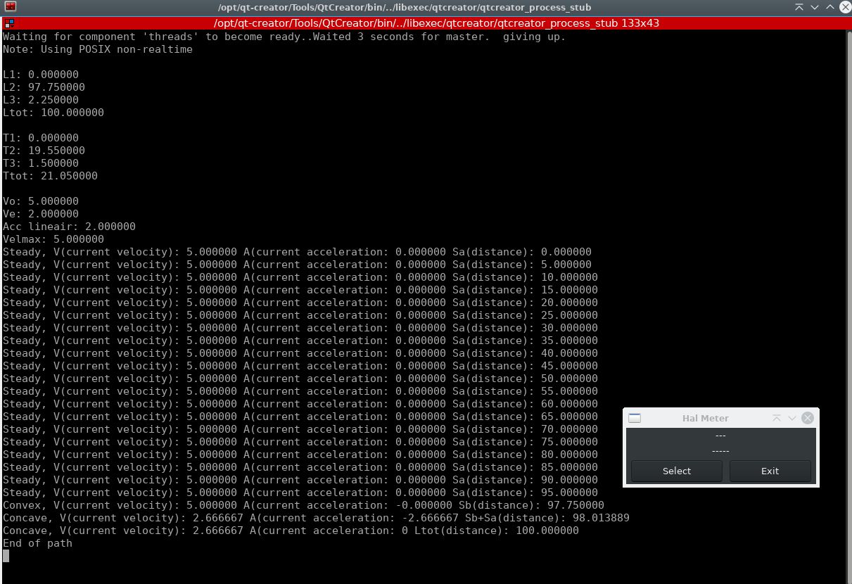
Here a function input as :

scurve(5,  // velmax
               2,   // accmax
               5,   // vo
               2,   // ve
               0,   // xs
               0,   // ys
               0,   // zs
               100, // xe
               0,   // ye
               0,   // ze
               1, // time output resolution in sec, for example 0.001 is a point every ms
               1);  // debug 0 or 1

Mention the output resolution is quite low at a 1 sec interval.

Last edit: 14 Jun 2021 15:41 by Grotius.

Please Log in or Create an account to join the conversation.

arvidb
Offline
Platinum Member

14 Jun 2021 16:08 - 14 Jun 2021 16:10 #212034 by arvidb

Replied by arvidb on topic LinuxCNC S-Curve Accelerations

Grotius wrote:
The plotted graph's at github show everything is printed ok when using vo and ve parameters.

I can't see any problem with the velocity plots at your github, however the position plots are not consistent with the velocity plots. All your position plots start and end horizontally (slope = 0), which they shouldn't if there is initial (or end) velocity, since velocity is equivalent to slope of the position curve.

Also plots 2, 3, and 4 all have discontinuities in the slope of the position plots ("kinks"), which means there is a step change in velocity, corresponding to infinite acceleration at those points. The position plot should be completely smooth even with acceleration-limited motion.

I have run into similar issues while developing my code, and in my testing I now double-check for such issues by differentiating the position output in several stages to get approximate velocity, acceleration and jerk values derived directly from the successive position outputs. I then check that these derived values doesn't deviate too much from the calculated ones at each time step. This automated test has been very useful to find bugs, and I can really recommend it!

Last edit: 14 Jun 2021 16:10 by arvidb.

Please Log in or Create an account to join the conversation.

Grotius
Offline
Platinum Member

14 Jun 2021 17:23 #212039 by Grotius

Replied by Grotius on topic LinuxCNC S-Curve Accelerations

Hi Arvidb,

Also plots 2, 3, and 4 all have discontinuities in the slope of the position plots ("kinks"),
This are no position plots ! ( Grey lines ).
It are scurve rendement curves.
A horizontal grey curve is no progress or travel, no rendement in travel.
With a max slope (steep curve) the rendement of the scurve implementation is at is best.
A kink in the plot show's a transition to a different scurve rendement. This is nothing special or to worry about.
The grey line is scaled at y axis : scale=0.15 to fit the plot.

curveup (// Be aware graphicsview is inverted on y-axis.)
concave period : ellipse = scene->addEllipse(T, scale*(Sa*-1), 0.1, 0.1, GreyPen);
convex period : ellipse = scene->addEllipse(T, scale*((Sa+Sb)*-1), 0.1, 0.1, GreyPen);
curvesteady
ellipse = scene->addEllipse(T, scale*(S*-1), 0.1, 0.1, GreyPen);
curvedown
convec period : ellipse = scene->addEllipse(T, scale*(Sb*-1), 0.1, 0.1, GreyPen);
concave period: ellipse = scene->addEllipse(T, scale*((Sb+Sa)*-1), 0.1, 0.1, GreyPen);

Please Log in or Create an account to join the conversation.

arvidb
Offline
Platinum Member

14 Jun 2021 17:54 #212041 by arvidb

Replied by arvidb on topic LinuxCNC S-Curve Accelerations

Rendement? I don't know what that means. (Is it french? "Yield" or "Output"? I still don't know what that means in this context.)

You write on your github page: "Grey = Travelled in time". And you write in an earlier post in this thread that "Grey is S (distance) versus T (time)." I would call this (relative) position?

If you have a "kink" in "distance travelled versus time", that means you have a discontinuity in velocity and thus infinite acceleration at that point. And "distance travelled versus time" should always have a slope equal (or proportional, with scaling) to the velocity, or something is wrong with the calculation of either velocity or (relative) position.

If I'm misunderstanding what the grey curve is, can you add a plot of (relative & scaled) position to your graphs? That is the most important output from a motion planner after all.

Please Log in or Create an account to join the conversation.

Grotius
Offline
Platinum Member

14 Jun 2021 19:39 - 14 Jun 2021 19:50 #212052 by Grotius

Replied by Grotius on topic LinuxCNC S-Curve Accelerations

Hi Arvidb,

Rendement is like "the effectiveness".

I made a short video about the scurve graph.
user-images.githubusercontent.com/448801...7d6-c7dcf68d7db7.mp4

The grey line is now showing time versus displacement for point in x direction, to simplify it.
Point x is from x0 to ~x100mm in the video.

(ellipse = scene->addEllipse(T, p.x*-1*scale, 0.1, 0.1, GreyPen);
scale=0.15;

This is how it should look like :

In a normal situation we see a displacement as in above graph.
When doing exotic's we can end up with so called "kink" in the displacement curve.

Arvidb, In your point of view this "kink" is a bad thing? I don't have something like it's a bad thing.

Last edit: 14 Jun 2021 19:50 by Grotius.

Please Log in or Create an account to join the conversation.

arvidb
Offline
Platinum Member

14 Jun 2021 21:30 - 14 Jun 2021 21:47 #212059 by arvidb

Replied by arvidb on topic LinuxCNC S-Curve Accelerations

Yes, Grotius, in my view the kink is a bad thing. To the left of the kink you are moving at one velocity, to the right of the kink you are moving at another velocity == step change in velocity == infinite acceleration == possible damage to CNC machine (and a very surprised operator) == bad thing.

Velocity is change in displacement over time, right? That is, v = Δs/Δt = the derivate of displacement.

You can approximate the true velocity of something moving along your grey displacement curve by differentiation:

true_vel = (S - S_prev)/timeresolution;
S_prev = S;

Add a plot of true_vel to your graphs and you'll see what I mean.

Last edit: 14 Jun 2021 21:47 by arvidb.

Please Log in or Create an account to join the conversation.

Grotius
Offline
Platinum Member

14 Jun 2021 22:09 - 14 Jun 2021 22:33 #212061 by Grotius

Replied by Grotius on topic LinuxCNC S-Curve Accelerations

Hi Arvidb,

Do you have an idea how the lecture dealing with this "kink" in the curve, you would expect researchers have dealed with this
before?

It's quite hard to imagine when the velocity curve looks ok and the acceleration curve looks ok.
There could be a kink in the displacement curve in some "exotic" cases.
[edit] After some experimenting it occur's when intitial and or end velocity is not zero.

And that this "kink" is in fact a infinite acceleration stage. When using a 20Kw servo it could result in a machine shock. :pinch:

Is it a idea to avoid this "kink" with a algoritme?

Are you able to implement your example in the qt code?

Last edit: 14 Jun 2021 22:33 by Grotius.

Please Log in or Create an account to join the conversation.

Time to create page: 0.148 seconds

LinuxCNC S-Curve Accelerations

Attachments:

Attachments:

Attachments: